In many areas of physical science, the need to establish a relationship between an independent variable, and a dependent variable, based on experimental data arises. This is defined as “Regression” Analysis, a term first mentioned in 1885 by Sir Francis Galton. For this, the traditional method would be to plot data points on a graph sheet and draw an estimated curve. If this curve is almost a straight line, we say that there is a linear relationship between the two variables. The study of variables that are thought to be showing such a relationship takes a separate field known as Linear Regression Analysis. Nowadays, we can use software programs to make this process more accurate and easier as well. The Least Square Fitting method is a form of Linear Regression Analysis.

The main expectation here is for the deviation between the predicted points and the experimental points to be minimum. An important assumption of this method is that the independent variable recordings don’t contain errors. Errors are considered only for the dependent variable recordings.

Graphical Representation

Consider a scatter of data on an x-y plane where x is the independent and y is the dependent variable. Let y = a + bx be the regressed line depicting a relationship between these two variables. Coefficients a and b are to be determined using the Least Squares Fitting method. The figure below shows the data points in blue crosses (as y_i‘s). The regressed line is given in orange and the regressed points as black dots (y‘s).

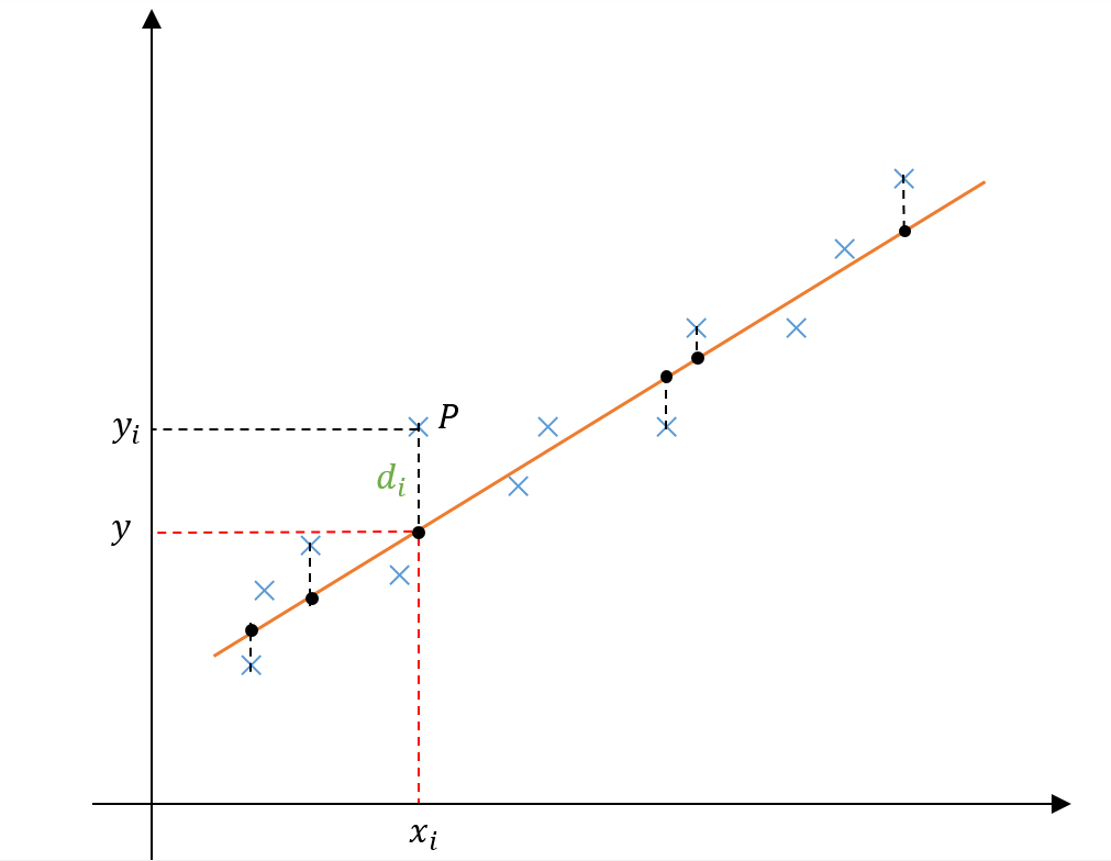
Consider a data point given by P = (x_i, y_i). The vertical distance between this point and the y-value corresponding to x_i on the regressed line is d_i. We can see from the figure that d_i = y_i – y = y_i – (a + bx_i). This value can be either positive or negative depending on the position of the data point with respect to the regressed line. We can make d_i a positive quantity by squaring or taking the absolute value. Let’s consider the square of d_i in our calculations.

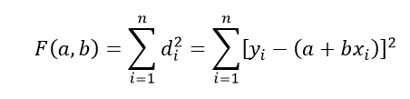
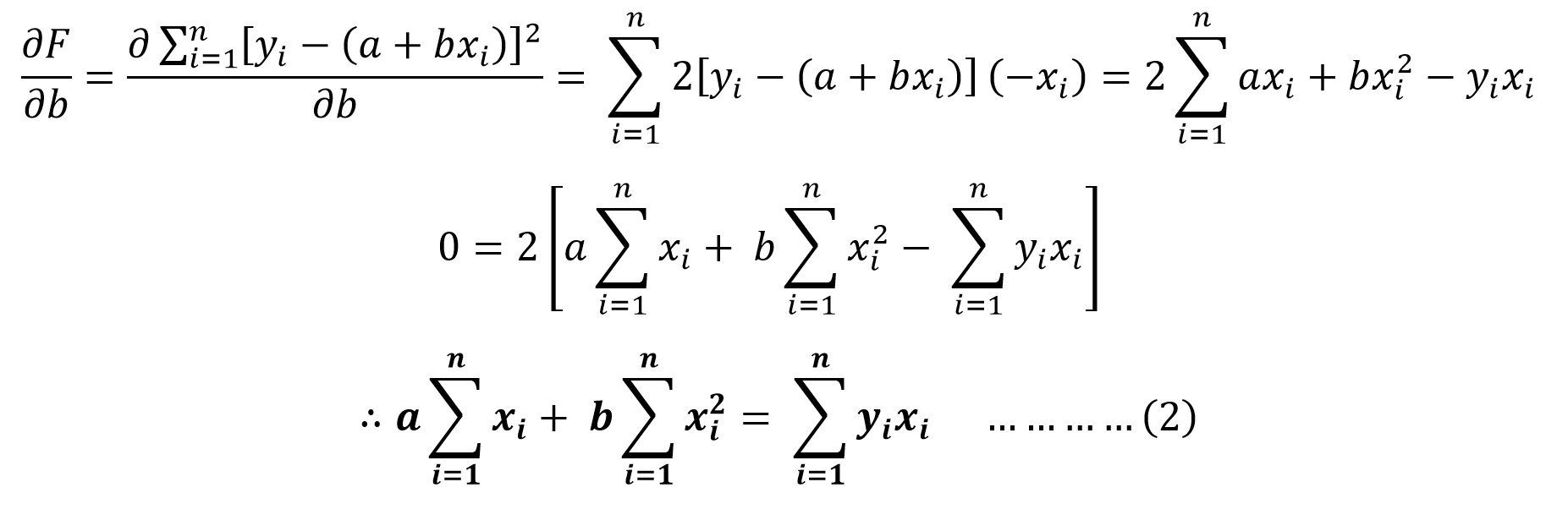
Now taking the summation of the distance from each data point to the relevant point in the regressed curve as F(a,b) we can obtain the following expression.

LEAST Square Fitting

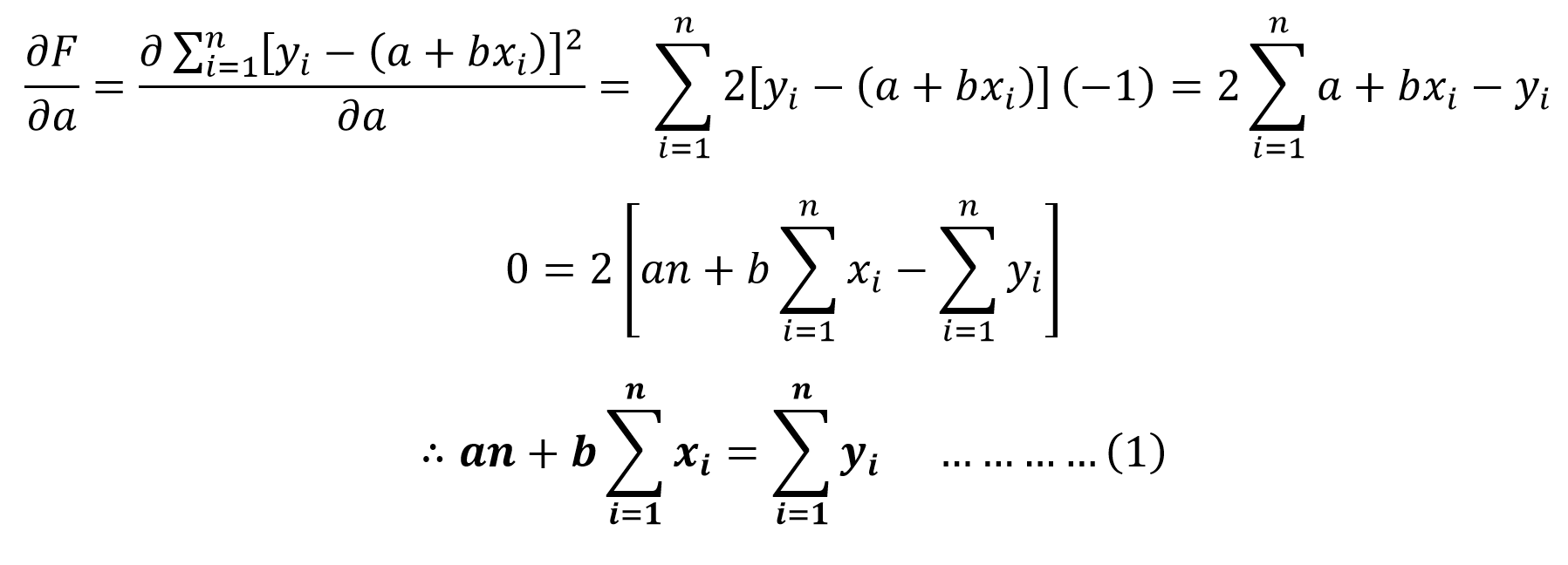
The emphasis on the term “least” shows the need to differentiate the function F(a,b) with respect to a and b. We can then equal these two expressions to 0 and simplify. This results in finding the coefficients a and b giving the minimum deviation between the data points and regressed points. 

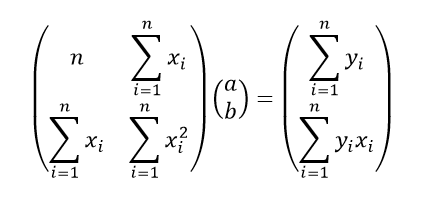
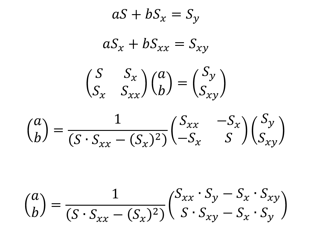
By considering (1) and (2) above we can then represent this as a linear system of equations for a and b using matrices as below.

Consider the below arbitrary system where the coefficient matrix A_2×2 is invertible.

A_2×2 . X_2×1 = B_2×1 

A^-1_2×2 . A_2×2 . X_2×1 = A^-1_2×2 . B_2×1 

I_2×2 . X_2×1 = A^-1_2×2 . B_2×1 

X_2×1 = A^-1_2×2 . B_2×1 

We can apply this to the derived system and obtain an expression for the coefficients.

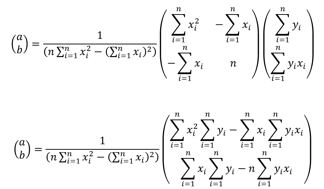
Thus, we can compute a and b and obtain a linear regression of two variables using the Least Square Fitting method.

Adding in Errors

We carry out the above derivation by assuming that the error in the measurement of the independent variable is uniform. However, in most cases that is not true. Due to varying sensitivities of measuring instruments, the error measurements vary as well.

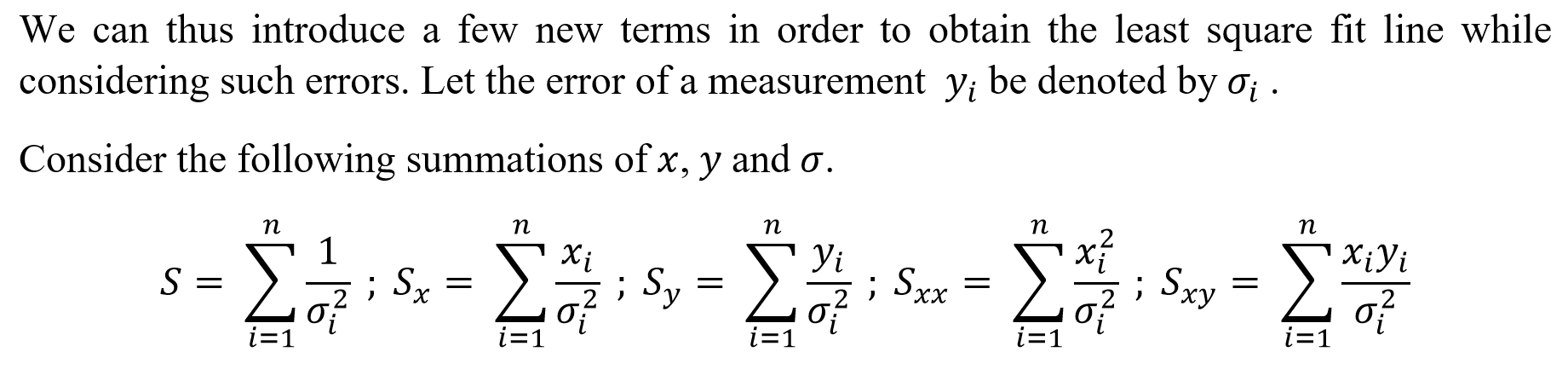
We can obtain two linear equations with a and b and represent them as a system of matrices in the same manner done previously.

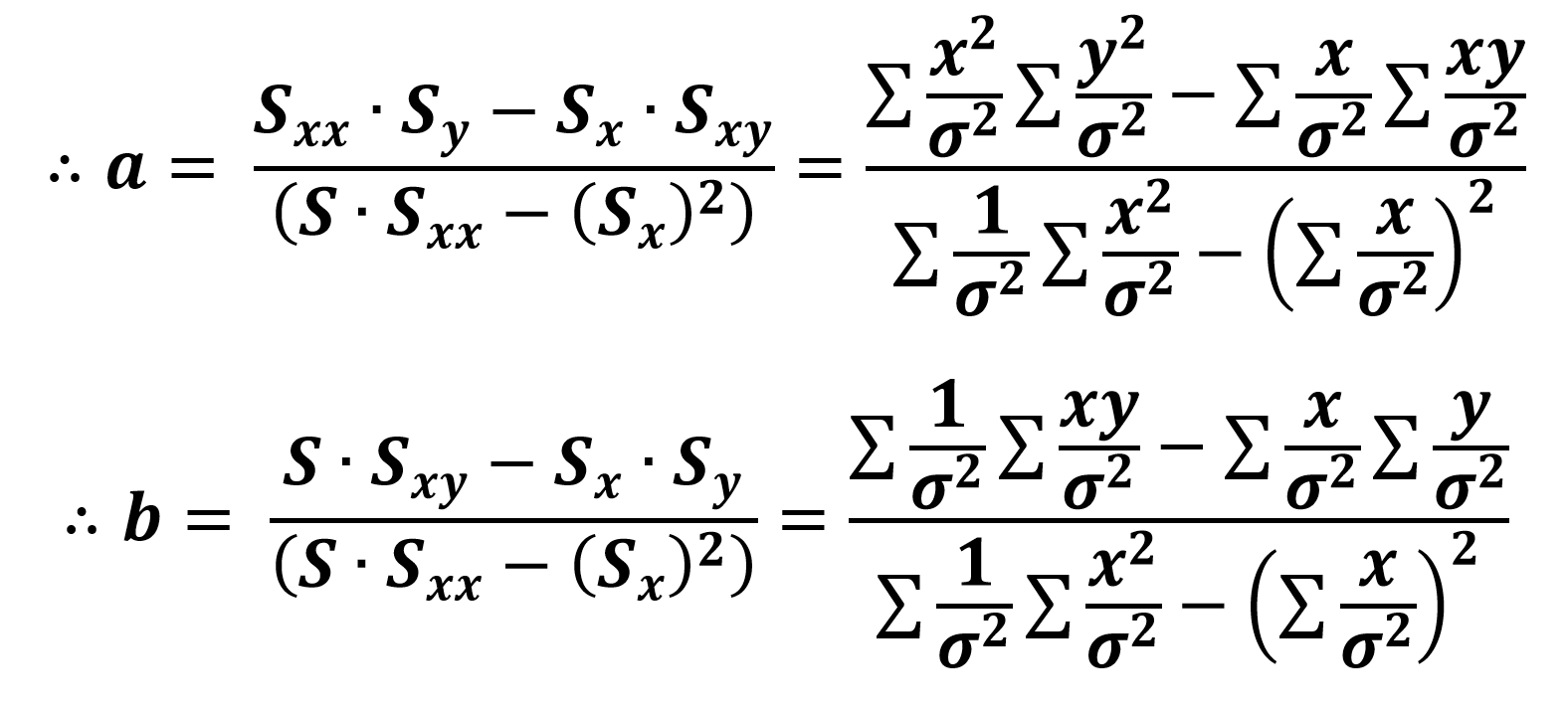
We can observe closely and see that this gives the same formulas for a and b as in the previous case if we take the errors to be constant, thus canceling out the term from the expressions.

Computations: Too many? Or made easy?

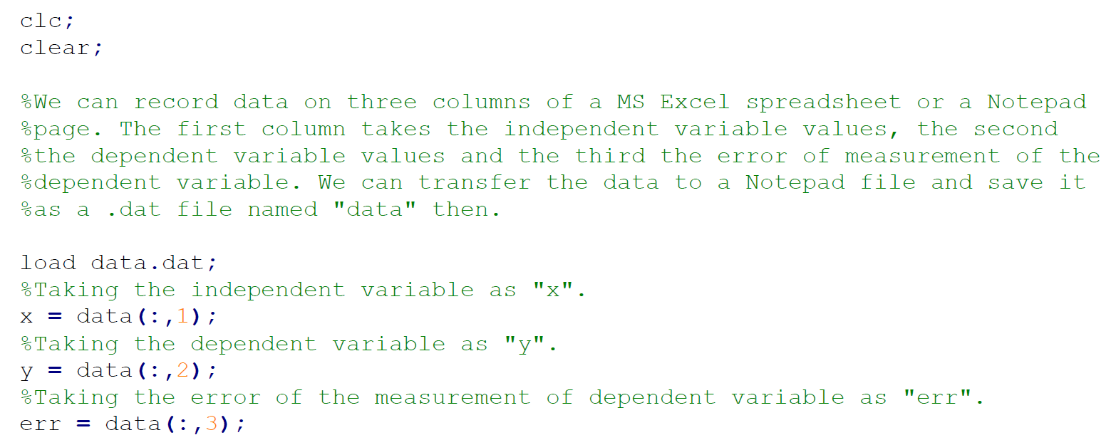
This all depends on the experiment conduct and the number of data points we record. For an experiment with 6 – 10 data points using a scientific calculator for the Least Square Fit method seems manageable. But, for those involving 20, 50, or more data points it seems to be very impossible. Thus, we use the magic of computers. While MS Excel is a very capable software in this aspect, software like MATLAB and Octave are widely used for mathematical analysis and modeling. Let’s take a look at the MATLAB codings for this.

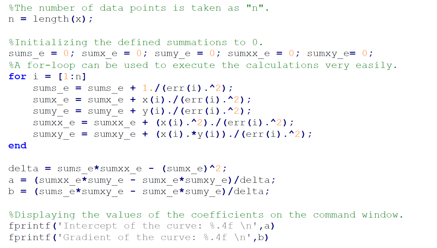
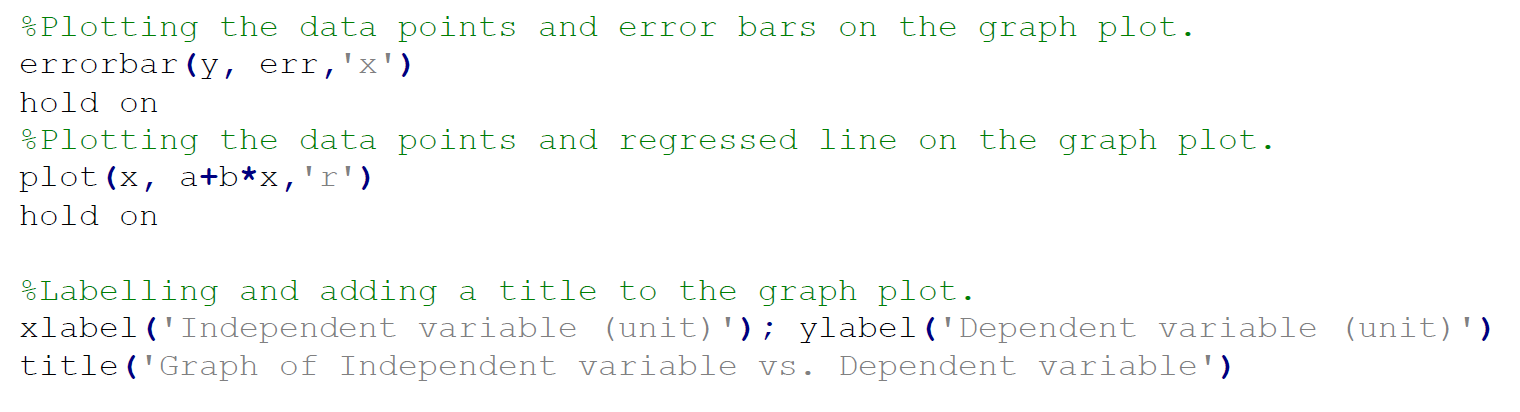
Therefore, we see that we can quite quickly compute and plot a line regressed using the Least Squares Fitting method using MATLAB. But, is this it? While easier than using a calculator, can we make this more efficient?

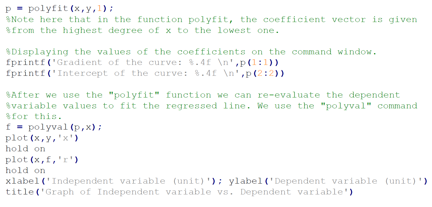
polyfit(x, y, 1)

In order to make things easier, MATLAB has a built-in solution for this. This whole code could be implemented using a single command: polyfit(independent variable values matrix, dependent variable values matrix, order of polynomial).

This command fits a polynomial of a specific order to a set of data points and stores the coefficients in a matrix. Since we’re discussing Linear regression, we can set the order as 1. This single command performs the calculations of the Least Square Fitting method of Linear Regression to extreme accuracy and efficiency.

Thus, we see a great example of how computers and software can be used to facilitate analysis.

References:

01. Anon., n.d. Simple Linear Regression Analysis. [Online] Available at http://home.iitk.ac.in/~shalab/econometrics/Chapter2-Econometrics-SimpleLinearRegressionAnalysis.pdf

02. Chasnov, J. R., 2012. Numerical Methods. [Online] Available at https://www.math.ust.hk/~machas/numerical-methods.pdf

03. Miller, S. J., n.d. The Method of Least Squares. [Online] Available at https://web.williams.edu/Mathematics/sjmiller/public_html/BrownClasses/54/handouts/MethodLeastSquares.pdf

Featured Image Courtesy: https://bit.ly/3adE1iY